DFT

Overview

JARVIS-DFT is a density functional theory-based database for ~40000 3D, ~1000 2D materials and around a million calculated properties. JARVIS-DFT mainly uses vdW-DF-OptB88 functional for geometry optimization. It also uses beyond-GGA approaches, including Tran-Blaha modified Becke-Johnson (TBmBJ) meta-GGA, PBE0, HSE06, DMFT, G0W0 for analyzing selective cases. In addition to hosting conventional properties such as formation energies, bandgaps, elastic constants, piezoelectric constants, dielectric constants, and magnetic moments, it also contains unique datasets, such as exfoliation energies for van der Waals bonded materials, spin-orbit coupling spillage, improved meta-GGA bandgaps, frequency-dependent dielectric function, spin-orbit spillage, spectroscopy limited maximum efficiency (SLME), infrared (IR) intensities, electric field gradient (EFG), heterojunction classifications, and Wannier tight-binding Hamiltonians. These datasets are compared to experimental results wherever possible, to evaluate their accuracy as predictive tools. JARVIS-DFT introduces protocols such as automatic k-point convergence that can be critical for obtaining precise and accurate calculation results.

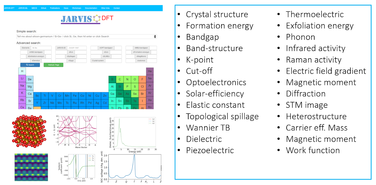
Table. A brief summary of datasets available in the JARVIS-DFT.

Material classes	Numbers
3D-bulk	33482
2D-bulk	2293
1D-bulk	235
0D-bulk	413
2D-monolayer	1105
2D-bilayer	102
Molecules	12
Heterostructure	3
Total DFT calculated systems	37646

Table. A brief summary of functionals used in optimizing crystal geometry in the JARVIS-DFT.

Functionals	Numbers
vdW-DF-OptB88 (OPT)	37646
vdW-DF-OptB86b (MK)	109
vdW-DF-OptPBE (OR)	111
PBE	99
LDA	92

Table. A brief summary of material-properties available in the JARVIS-DFT. The database is continuously expanding.

JARVIS-DFT Properties	Numbers
Optimized crystal-structure (OPT)	37646
Formation-energy (OPT)	37646
Bandgap (OPT)	37646
Exfoliation energy (OPT)	819
Bandgap (TBmBJ)	15655
Bandgap (HSE06)	40
Bandgap (PBE0)	40
Bandgap (G0W0)	15
Bandgap (DMFT)	11
Frequency dependent dielectric tensor (OPT)	34045
Frequency dependent dielectric tensor (TBmBJ)	15655
Elastic-constants (OPT)	15500
Finite-difference phonons at Г-point (OPT)	15500
Work-function, electron-affinity (OPT)	1105
Theoretical solar-cell efficiency (SLME) (TBmBJ)	5097
Topological spin-orbit spillage (PBE+SOC)	11500
Wannier tight-binding Hamiltonians (PBE+SOC)	1771
Seebeck coefficient (OPT, BoltzTrap)	22190
Power factor (OPT, BoltzTrap)	22190
Effective mass (OPT, BoltzTrap)	22190
Magnetic moment (OPT)	37528
Piezoelectric constant (OPT, DFPT)	5015
Dielectric tensor (OPT, DFPT)	5015
Infrared intensity (OPT, DFPT)	5015
DFPT phonons at Г-point (OPT)	5015
Electric field gradient (OPT)	15187
Non-resonant Raman intensity (OPT, DFPT)	250
Scanning tunneling microscopy images (PBE+SOC)	770

Methodology

Input structure

The initial/input crystal structures were obtained from the Inorganic Crystal Structure Database, Materials Project, OQMD, AFLOW, COD databases. These input structures are then subjected to a set of geometric and electronic optimizations (discussed below) following JARVIS-DFT workflow protocols. After the geometric optimization, several materials properties are calculated .

# Make sure JARVIS_VASP_PSP_DIR is correctly set for VASP pseudopotentials.
from jarvis.io.vasp.inputs import Poscar
from jarvis.tasks.vasp.vasp import JobFactory
p = Poscar.from_file("POSCAR")
print (p)
JobFactory().all_optb88vdw_props(mat=p)

Geometric optimzation

DFT calculations were carried out using the Vienna Ab-initio simulation package (VASP) software using the workflow given on our JARVIS-Tools github page (https://github.com/usnistgov/jarvis). We use the projected augmented wave method . Both the internal atomic positions and the lattice constants are allowed to relax in spin-unrestricted calculations until the maximal residual Hellmann–Feynman forces on atoms are smaller than 0.001 eV Å−1 and energy-tolerance of 10-7 eV with accurate precision setting (PREC=Accurate). Note that force convergence is important for properties such as phonons, elastic constants etc. We use spin-polarized set-up with initial magnetic moment of default value 1 muB during geometric optimization. Also use conjugate gradient algorithm for ionic relaxation (IBRION=2).

Functional selection

We mainly use OptB88vdW method for our calculations, but we also carryout local density approximation (LDA) and generalized gradient approximation with Perdew-Burke-Ernzerhof (GGA-PBE)-based calculations for benchmarking purposes. OptB88vdW functional, has been shown to gives accurate lattice parameters for both van der Waals (vdW) and non-vdW solids. TBmBJ potential is used as a meta-GGA method for better predicting the bandgaps and dielectric function of a material on the OptB88vdW optimized cell.

from jarvis.tasks.vasp.vasp import GenericIncars
pbe = GenericIncars().pbe()
optb88vdw = GenericIncars().optb88vdw()
lda = GenericIncars().lda()

K-point and cut-off convergence

We use the Monkhorst-Pack scheme to generate k-points, but after the generation, the grid is shifted so that one of the k-points lies on the Г-point. We included the gamma-point because we were interested in computing quantities that require gamma-point contribution, such as optical transition for our optoelectronic database, gamma-point phonons for our elastic properties, finding multiferroic materials which have negative phonons at the gamma-point. The k-points are continuously stored in memory, to check that each of the new k-points generated by equation is unique. The k-points line density starts from length 0, with Г-point being the only k-point and is increased by 5 Å at each successive iteration if the difference between the energy computed with the new k-points and the one computed with previous k-points is more than the tolerance. After the convergence with a particular tolerance, we compute five extra points to further ensure the convergence. This procedure is repeated until convergence is found for all 5 extra points. A similar convergence procedure is carried out for the plane wave cut-off until the energy difference between successive iterations is less than the tolerance for 6 successive points. The plane wave cut-off is increased by 50 eV each time, starting from 500 eV. In both convergence procedures, we perform only single step electronic relaxation, i.e. no ionic relaxation is considered. When starting the cut-off energy convergence, we used a minimal k-point length of 10 Å. Similarly, for the k-point convergence we started with a cut-off of 500 eV. We used Gaussian smearing (with 0.01 eV parameter) which is recommended by several DFT codes, because it is less sensitive than other methods to determine partial occupancies for each orbital. This leads to an easier DFT-SCF convergence, especially when the materials are not apriori known to be a metal or insulator, which is always the case in this work. However, it is to be emphasized that, in principle, k-points and smearing parameters should be converged together, but this requires a very computationally expensive workflow. For this reason, we choose to converge k-points and cut-off only. In addition to the above convergence procedure, we further increase the cut-off by 30% for elastic, dielectric and electric field gradient, piezoelectric tensors as the volume and shape of the material may change during the distortions.

optb88 = GenericIncars().optb88vdw()
job = JobFactory(use_incar_dict=optb88.incar, pot_type=optb88.pot_type)
encut = job.converg_encut(mat=mat)
length = job.converg_kpoint(mat=mat)
energy, contcar_path = job.optimize_geometry(
            mat=mat, encut=encut, length=length
)

DFT+U

DFT+U corrections are used only for special cases because it is somewhat tricky to get formation energies from the total energies obtained from such calculations. DFT+U calculations are used during magnetic topologic insulator search cases mainly. We generally use U=3.0 eV or complete U-scan (0 to 3 eV) for enumerating the effects of U-parameter.

from jarvis.io.vasp.inputs import find_ldau_magmom
atoms=Atoms.from_poscar('POSCAR')
ld_soc = find_ldau_magmom(atoms=atoms,lsorbit=True)
ld_nonsoc = find_ldau_magmom(atoms=atoms,lsorbit=False)

Spin-orbit coupling

Spin-orbit coupling usually split states that are degenerate in a nonrelativistic description. We consider spin-orbit coupling (LSORBIT = .TRUE.) only during spin-orbit spillage calculations for topological materials but not during geometric optimization or any other major property calculations. We take into account only scalar relativistic effects. Accurate lattice-constants of materials with vdW bonding can play a critical role in predicting the correct topology, as emphasized. We calculate the spillage using the Perdew, Burke and Ernzerhof (PBE) functional and 1000/atom k-points, as well as by analyzing the spillage along a high-symmetry Brillouin-zone path, with a 600 eV plane-wave cut-off.

Beyond DFT methods

JARVIS-DFT contains data using conventional local and semi-local methods, as well as beyond conventional DFT based methods such as meta-GGA (TBmBJ), G0W0, HSE06, PBE0, DMFT etc. BDFT methods are used to better predict electronic bandgaps, dielectric functions hence solar-cell efficiencies, as well magnetic moment (using DMFT) of a material. HSE06 and PBE0 were used to predict accurate bandgaps for exfoliable bulk and corresponding monolayer materials. We utilized two hybrid functionals: PBE0 and HSE06. In PBE0 the exchange energy is given by a 3:1 ratio mix of the PBE and Hartree–Fock exchange energies, respectively, while the correlation is completely given by the PBE correlation energy. In HSE (Heyd–Scuseria–Ernzerhof), the exchange is given by a screened Coulomb potential, to improve computational efficiency. An adjustable parameter (ω) controls how short range the interaction is. HSE06 is characterized by ω=0.2, while for a choice of ω=0 HSE becomes PBE0.

Density functional perturbation theory

We carry out the Density functional perturbation theory (DFPT) (as implemented in the VASP code, IBRION=8) calculation on the standard conventional cell for each material. We determine the Born-effective charge, piezoelectric and dielectric (ionic+electronic parts) tensors and the phonon eigenvectors. DFPT is also used to calculate Infrared and Raman intensities for selected materials. As mentioned earlier, it is important to converge K-points, cut-off and parameters to get reliable results which is taken into account in the JARVIS-DFT.

Finite-difference method

The elastic tensor is determined by performing six finite distortions of the lattice and deriving the elastic constants from the strain-stress relationship. In addition to elastic tensor, the finite difference (IBRION=6) method used predicts the phonons at gamma-point for the conventional cell used.

Linear Optics

To obtain the optical properties of the materials, we calculated the imaginary part of the dielectric function from the Bloch wavefunctions and eigenvalues (neglecting local field effects) (LOPTICS=.TRUE.). We introduced three times as many empty conduction bands as valance bands. This treatment is necessary to facilitate proper electronic transitions. We choose 5000 energy grid points to have a sufficiently high resolution in dielectric function spectra. Several properties such as absorption coefficient, solar-cell efficiency, and reflectivity can be predicted with the dielectric function data. Note that due to bandgap underestimation the peaks may beshifted. A better method such as TBmBJ, HSE06, G0W0 is necessary for predicting better behavior.

Wannierization

We use Wannier90 to construct Maximally-Localized Wannier Functions (MLWF) based TB-Hamiltonians. For the case of interest in this work, where we wish to describe both the valence and conduction bands near the Fermi level, it is necessary to first select a set of bands to Wannierize, which includes separating the conduction bands from the free-electron-like bands that generally overlap with them in energy. The procedure to determine this localized subspace of Bloch wavefunctions proceeds similarly to minimization described above, where after an initial guess, the subspace is iteratively updated in order to minimize the spread function. After this initial disentanglement step, the Wannierization of the selected subspace proceeds as described above. Due to the iterative non-linear minimization employed during both the disentanglement and Wannierization steps, the localization and utility of the final Wannier functions depend in practice on the initial choice of orbitals that are used to begin the disentanglement procedure, and which are then used as the initial guess for the Wannierization. Our initial guesses consist of a set of atomic orbitals we have chosen to describe all the chemically relevant orbitals for each element in typical elemental systems and compounds.

During the disentanglement step, it is possible to choose an energy range that is included exactly (“the frozen window”), with the result that the Wannier band structure will exactly match the DFT band structure in this energy range and at the grid of k-points used in the Wannierization. We use a frozen window of ± 2 eV around the Fermi-energy. This window ensures that bands near the Fermi level are well described by the WTBH. For cases where the original WFs were unsatisfactory (see below), we found that lowering the lower bound of this window to include all of the valence bands often improves that WTBH, which we use as a second Wannierization setting. In order to validate our WTBH, we calculate the maximum absolute difference (μ) between the Wannier and DFT eigenvalues within an energy range of ± 2eV around the Fermi level.

A weakness of this evaluation method is that highly dispersive energy bands (high (dE_nk)/dk) can result in high μ values even if the WTBH is of good quality because any slight shift in the k-direction of a dispersive band will result in a large energy error. We consider that systems with μ less than 0.1 eV to useful for most applications, and we provide data for the user to evaluate individual WTBH for their own applications.

from jarvis.io.wannier.inputs import Wannier90win
box = [[2.715, 2.715, 0], [0, 2.715, 2.715], [2.715, 0, 2.715]]
coords = [[0, 0, 0], [0.25, 0.25, 0.25]]
elements = ["Si", "Si"]
Si = Atoms(lattice_mat=box, coords=coords, elements=elements)
Wannier90win(struct=Si, efermi=0.0).write_win(name=win)

Boltzmann transport

The transport properties were calculated using the Boltzmann transport equation (BTE) implemented in the BoltzTrap code. The BTE is used to investigate the non-equilibrium behavior of electrons and holes by statistically averaging all possible quantum states. The computation of the relaxation time is very computationally expensive, especially in a high-throughput context, hence a constant relaxation time approach is used here.

from jarvis.tasks.boltztrap.run import run_boltztrap
path = 'xyz'
run_boltztrap(path)

Partial charge density

The partial charge densities are used to calculate scanning tunneling microscopy images. The surface charge and probability densities are calculated by integrating the local density of states function (ILDOS) over an energy range of ±0.5 eV from the conduction band minima (CBM) to Fermi energy (EF) and valence band maxima (VBM) to Fermi energy (EF). The STM images are calculated using Tersoff-Hamann approach.

Property Details

Atomic structure and derived properties

After obtaining the initial structures from several databases, we optimize following JARVIS-DFT protocols of a) converging k-points, b) converging cut-off, c) converging energy, d) converging forces. These final optimized structures are analyzed in terms of scalar quantities such as density, volume etc. as well as statistical functions such as radial distribution function, angular distribution function, dihedral distribution function, X-ray diffraction pattern etc. to know about the local atomisitic environments that controls several material-properties.

from jarvis.core.atoms import Atoms
from jarvis.analysis.structure.neighbors import NeighborsAnalysis
from jarvis.ai.descriptors.cfid import CFID
from jarvis.analysis.diffraction.xrd import XRD
from jarvis.analysis.structure.spacegroup import Spacegroup3D

box = [[2.715, 2.715, 0], [0, 2.715, 2.715], [2.715, 0, 2.715]]
coords = [[0, 0, 0], [0.25, 0.25, 0.25]]
elements = ["Si", "Si"]
atoms = Atoms(lattice_mat=box, coords=coords, elements=elements)
density = round(density,2)


spg = Spacegroup3D(atoms)
prim_atoms = spg.primitive_atoms
conv_atoms = spg.conventional_standard_structure
spg_numb = spg.space_group_number
crys_system = spg.crystal_system
conv_params = conv_atoms.lattice.parameters

packing_fr = round(atoms.packing_fraction, 3)

nbr = NeighborsAnalysis(atoms)
rdf_bins, rdf_hist, nn = nbr.get_rdf()
nbr = NeighborsAnalysis(atoms, max_cut=10.0)
ang1_hist, ang1_bins = nbr.ang_dist_first()
ang2_hist, ang2_bins = nbr.ang_dist_second()
dhd_hist, dhd_bins = nbr.get_ddf()

two_thetas, d_hkls, intensities = XRD().simulate(atoms=atoms)

cfid = CFID(atoms).get_comp_descp()

Formation energy

The enthalpy of formation is the standard reaction enthalpy for the formation of the compound from its elements (atoms or molecules) in their most stable reference states. We report formation energies at 0K only based on energies directly obtained from the DFT especially with OptB88vdW functional. We have calculated the elemental energies (in respective crystalline forms) and treat those energies as the chemical potential. These chemical potentials are subtracted from the total energies of the system to predict the formation energies. If functional other than OptB88vdW is used then the unary energy needs to be provided.

from jarvis.analysis.thermodynamics.energetics import form_enp
total_energy = -9.974648
fen = form_enp(atoms=atoms, total_energy=total_energy)

Exfoliation energies

The exfoliation energy for 2D materials is computed as the energy difference per atom for bulk and monolayer systems.

Defect formation energies

Defect formation energies are available for a few 2D materials. For neutral defect formation energies, we generate a at least 11 Angs. Cell for 2D materials and create point defects using unique Wyckoff information. The total energy of the defect system, the energy of the perfect 2D crystal and the elemental chemical potential is then used to predict the defect formation energies. Currently this property is available for OptB88vdW functional only.

from jarvis.analysis.thermodynamics.energetics import get_twod_defect_energy
from jarvis.io.vasp.outputs import Vasprun
tmp_xml=os.path.join(os.path.dirname(__file__), "JVASP-667_C_C_c.xml")
vrun=Vasprun(tmp_xml)
Ef=get_twod_defect_energy(vrun=vrun,jid="JVASP-667",atom="C")

Electronic density of density of states

EDOS is a spectrum of the number of allowed electron energy levels (occupied and unoccupied) against energy interval (generally in electron volt). EDOS is generally calculated based on a dense k-point grid with a smoothening/smearing setup. EDOS is generally rescaled with respect to the Fermi-energy of the system. A high value for the DOS represents a high number for the electronic states that can be occupied. Experimental methods such as scanning tunneling microscopy can be used obtain EDOS. One of the obvious properties that can be calculated from EDOS is the bandgap. EDOS can be based on total density of states or further resolved into atom-projected and element-projected density of states. The projected EDOS provides information about the particular electronic orbitals (say s,p,d,f) and specific atom (say Si) contributing towards a particular energy level. We calculate EDOS for both semi-local, HSE06 and PBE0 methods. At least, DOS is provided at local or semilocal materials for all the materials.

from jarvis.io.vasp.outputs import Vasprun
vrun = Vasprun('vasprun.xml')
total_dos = vrun.total_dos
energies = total_dos[0]
spin_up = total_dos[1]
spin_dn = total_dos[2]
spdf_dos = vrun.get_spdf_dos()
atoms_dos = vrun.get_atom_resolved_dos()

Electronic Bandstructure

Following the laws of quantum mechanics only certain energy levels are allowed and others could be forbidden. These levels can be discrete or spilt, called bands. Electronic bands depend on crystal momentum leading to bandstructure. The allowed states which are filled (upto the Fermi level) are valence bands while the unoccupied bands are conduction bands. The difference in energy between the conduction and valence band gives rise to the bandgaps. The materials with no bandgap are termed metals, with low bandgap semiconductors and with high bandgaps insulators. We calculate bandstructure using local, semi-local as well as hybrid functionals.

from jarvis.io.vasp.outputs import Vasprun
vrun = Vasprun('vasprun.xml')
band_info = vrun.get_bandstructure(kpoints_file_path='KPOINTS')

Spin-orbit spillage and topological properties

Topological materials driven by spin-orbit coupling have different bandgaps with/without spin orbit coupling effects. Spillage is calculated by comparing the wavefunctions of these two bandstructures. We calculate the spillage values for a large set of low bandgap and high atomic mass materials, with a spillage value of 0.5 as a threshold to screen for potential topologically non-trivial materials. The threshold denotes number of band-inverted electrons. This criterion can be used for predicting non-trivial topological behavior of metals, semiconductors and both perfect and defective structures.

from jarvis.analysis.topological.spillage import Spillage
spl = Spillage(wf_noso=wf_noso, wf_so=wf_so)
info = spl.overlap_so_spinpol()
max_spillage = round(info["spillage"], 2)

Frequency dependent dielectric function and optoelectronic properties

We use linear optics theory at semilocal and meta-GGA levels to calculate frequency dependent real and imaginary part of dielectric function. The meta-GGA based data should predict better bandgaps hence dielectric function. Note that ionic contributions are ignored in such calculations. Several important properties such as absorption coefficient, electron energy loss spectrum, reflectivity, solar cell efficiency etc. can be calculated from the frequency dependent dielectric function.

Using the absorption coefficient and bandgap (indirect and direct gaps), we calculate theoretical solar cell efficiencies of a material.

from jarvis.io.vasp.outputs import Vasprun
vrun = Vasprun('vasprun.xml')
reals, imags = vrun.dielectric_loptics
en, abz = lvrun.avg_absorption_coefficient
abz = abz * 100
eff_slme = SolarEfficiency().slme(
en, abz, indirgap, indirgap, plot_current_voltage=False
)
# print("SLME", 100 * eff)
eff_sq = SolarEfficiency().calculate_SQ(indirgap)
eff_slme = round(100 * eff_slme, 2)
eff_sq = round(100 * eff_sq, 2)

Static dielectric tensor

Dielectric materials are important components in many electronic devices such as capacitors, field-effect transistors computer memory (DRAM), sensors and communication circuits. Both high and low-value DL materials have applications in different technologies. Static dielectric constants with both ionic and electronic contributions are obtained using DFPT method. The electronic part of the dielectric constant is generally in close agreement with that obtained from the linear optics method mentioned above.

from jarvis.io.vasp.outputs import Vasprun
vrun = Vasprun('vasprun.xml')
epsilon = vrun.dfpt_data["epsilon"]["epsilon"]
epsilon_rpa = vrun.dfpt_data["epsilon"]["epsilon_rpa"]
epsilon_ion = vrun.dfpt_data["epsilon"]["epsilon_ion"]

Piezoelectric tensor

The piezoelectric effect is a reversible process where materials exhibit electrical polarization resulting from an applied mechanical stress, or conversely, a strain due to an applied electric field. Common applications for piezoelectricity include medical applications, energy harvesting devices, actuators, sensors, motors, atomic force microscopes, and high voltage power generation. PZ responses can be measured under constant strain, giving the piezoelectric stress tensor e_ij or constant stress, giving the piezoelectric strain tensor d_ij . Piezoelectric tensor is a 6x3 matrix.

from jarvis.io.vasp.outputs import Outcar
out = Outcar('OUTCAR')
pza = out.piezoelectric_tensor[1]
max_pza = np.max(np.abs(pza))
born_charges = vrun.dfpt_data["born_charges"]

Infrared intensity

The infrared intensity is important for thermal-imaging, infrared-astronomy, food-quality control. Infrared frequencies are classified in three categories: far (30-400 cm-1), mid (400-4000 cm-1) and near (4000-14000 cm-1) IR frequencies. The IR intensity is calculated obtained from the gamma-point phonon data used in the DFPT calculations.

from jarvis.analysis.phonon.ir import ir_intensity
from jarvis.io.vasp.outputs import Outcar, Vasprun
out = Outcar('OUTCAR')
vrun = Vasprun('vasprun.xml')
phonon_eigenvalues = out.phonon_eigenvalues
data = vrun.dfpt_data
phonon_eigenvectors = data["phonon_eigenvectors"]
masses = data["masses"]
born_charges = data["born_charges"]
x, y = ir_intensity(
      phonon_eigenvectors=phonon_eigenvectors,
      phonon_eigenvalues=phonon_eigenvalues,
      masses=masses,
      born_charges=born_charges,
)

Elastic tensor

We use finite difference method on conventional cells of systems for ET calculations. For bulk material, the compliance tensor can be obtained as the inverse.

Now, several other elastic properties calculated from Cij and sij. Some of the important properties are given below:

KV = ((C11+C22+C33) + 2(C12+C23+C31))/9

GV = ((C11+C22+C33) − (C12+C23 + C31) +3 (C44+C55+C66))/15

KR = ((s11+s22+s33) + 2(s12+s23+s31))-1

GR = 15(4(s11+s22+s33) - 4(s12+s23+s31) + 3(s44+s55+s66))-1

KVRH =(KV+KR)/2

GVRH =(GV+GR)/2

ν = (3KVRH − 2GVRH)/(6KVRH+2GVRH))

Here KV and GV are Voigt bulk and shear modulus, and KR and GR Reuss-bulk and shear modulus respectively. The homogenous Poisson ratio is calculated as ν. The EC data can be also used to predict the ductile and brittle nature of materials with Pugh (Gv/Kv) and Pettifor criteria (C12-C44) . Materials with Pugh ratio value >0.571 and Pettifor criteria <0 should be brittle, while materials with Pugh ratio value <0.571 and Pettifor criteria >0 should be ductile. For monolayer material calculations, the elastic tensor obtained from DFT code such as VASP, assumes periodic-boundary-condition (PBC). Therefore, cell vectors are used to calculate the area which again is used in computing stress. When dealing with the monolayer, an arbitrary vacuum padding is added in one of the direction (say z-direction). When computing EC we need to correct the output by eliminating the arbitrariness of the vacuum padding. We do that as a post-processing step by multiplying the Cij components (i,j≠3) by the length of the vacuum padding. Therefore, the units of EC turn into Nm-1 from Nm-2.

from jarvis.io.vasp.outputs import Outcar
from jarvis.analysis.elastic.tensor import ElasticTensor
cij = out.elastic_props)["cij"]
d = ElasticTensor(cij).to_dict()

From the associated finite-difference calculations, force constants (mainly at gamma point in our case) can be calculated. Using this information, we can predict the phonon density of states and bandstructure assuming the conventional cell used in the calculation is large enough (at least 11 Angstrom). Note that for smaller lengths the phonon bandstructure and density of states can show unreasonable frequencies at off and away from gamma points.

from jarvis.tasks.phonopy.run import run_phonopy
from jarvis.io.phonopy.outputs import bandstructure_plot
import yaml
run_phonopy('OUTCAR')
mesh_yaml = "mesh.yaml"
band_yaml = "band.yaml"
with open(mesh_yaml, "r") as f:
    doc = yaml.load(f)
nmodes = doc["phonon"][0]["band"]
ph_modes = []

for p in nmodes:
    ph_modes.append(p["frequency"])
ph_modes = sorted(set(ph_modes))
f = open(totdos, "r")
freq = []
pdos = []
for lines in f.readlines():
    if not str(lines.split()[0]).startswith("#"):
        freq.append(float(lines.split()[0]))
        pdos.append(float(lines.split()[1]))
frequencies, distances, labels, label_points = bandstructure_plot(band_yaml)

Thermoelectric properties

Thermoelectrics are materials that can convert a temperature gradient into electric voltage, or vice-versa. Themoelectrics can be used to regenerate electricity from waste heat, refrigeration and several other space-technology applications. The search for efficient thermoelectric materials is an area of intense research due the potential of converting waste heat into electrical power, and therefore improving energy efficiency and reducing fossil fuel usage.

from jarvis.io.boltztrap.outputs import BoltzTrapOutput  
from jarvis.tasks.boltztrap.run import run_boltztrap
path = 'xyz'
run_boltztrap(path)
all_data = BoltzTrapOutput(path).to_dict()

Wannier tight binding Hamiltonians

Wannier functions (WF) were first introduced in 1937, and have proven to be a powerful tool in the investigation of solid-state phenomenon such as polarization, topology, and magnetization. WTBH is not necessarily a material properties but can be useful in calculating several material properties. Mathematically, WFs are a complete orthonormalized basis set that act as a bridge between a delocalized plane wave representation commonly used in electronic structure calculations and a localized atomic orbital basis that more naturally describes chemical bonds. One of the most common ways of obtaining Wannier tight-bonding Hamiltonians (WTBH) is by using the Wannier90 software package to generate maximally localized Wannier functions, based on underlying density functional theory (DFT) calculations.

from jarvis.io.wannier.outputs import WannierHam
wann_ham = WannierHam(filename='wannier90_hr.dat')
vrun = "vasprun.xml"
bz = wann_ham.compare_dft_wann(vasprun_path=vrun, plot=False)

Scanning tunneling microscopy images

Since the invention of the scanning tunneling microscope (STM), this technique has become an essential tool for characterizing material surfaces and adsorbates. In addition to providing atomic insights, STM has been proven useful for characterizing the electronic structure, shapes of molecular orbitals, and vibrational and magnetic excitations. It can also be used for manipulating adsorbates and adatoms, and for catalysis and quantum information processing applications. We use Tershoff-Hamman approach to predict STM images of 2D materials.

from jarvis.analysis.stm.tersoff_hamann import TersoffHamannSTM
TH_STM = TersoffHamannSTM(chg_name='PARCHG')
t1 = TH_STM.constant_height(filename='STM.png')

Electric field gradients

EFG is a key parameter used to define Nuclear Quadrupole Resonance (NQR) spectral lines EFG is defined as the second derivative in Cartesian coordinates of the Coulomb potential at the nucleus position. By construction, the EFG, Vii is a traceless tensor. The coordinate system, in accordance with the convention used by experimentalists is chosen so that |V_zz |≥|V_yy |≥|V_xx |, which forces 0≤η<1. Note that if the point group of the site in question is cubic, then by symmetry all components are zero.

from jarvis.io.vasp.outputs import Outcar
efg = out.efg_raw_tensor
max_efg = np.max(np.abs(np.array(efg)))

DFT convergence parameters

Although density functional theory is exact in theory, its implementation requires several approximations such as the choice of basis-set, exchange-correlation functional, mesh-size for Brillouin zone (BZ) integration and plane-wave cut-off for plane-wave basis. These parameters need to be converged prior to geometric optimization and property predictions. Such convergences are performed for k-point and plane wave cut-off only in JARVIS-DFT leading to high quality of the data.

Data quality assessment

Method	#Materials	MAE (a)	MAE (b)	MAE (c)	RMSE (a)	RMSE (b)	RMSE (c)
OPT (All)	10052	0.11	0.11	0.18	0.29	0.30	0.58
PBE (All)	10052	0.13	0.14	0.23	0.30	0.29	0.61
OPT (vdW)	2241	0.20	0.21	0.44	0.44	0.44	0.99
PBE (vdW)	2241	0.26	0.29	0.62	0.45	0.51	1.09
OPT (non-vdW)	7811	0.08	0.08	0.11	0.23	0.24	0.39
PBE (non-vdW)	7811	0.09	0.09	0.12	0.22	0.25	0.36

Table: Comparison of bandgaps obtained from OPT functional and MBJ potential schemes compared with experimental results and DFT data available in different databases. Materials, space-group (SG), Inorganic Crystal Structure Database (ICSD#) id, Materials-Project (MP#) id, JARVIS-DFT id (JV#), bandgap from MP (MP), bandgap from AFLOW, bandgap from OQMD, our OptB88vdW bandgap (OPT), Tran-Blah modified Becke-Johnson potential bandgap (MBJ), Heyd-Scuseria-Ernzerhof (HSE06) and experimental bandgaps (eV) data are shown. Experimental data were obtained from 18,21,46,47__. MAE denotes the mean absolute error, while SC is the Spearman's coefficient.

Mats.	SG	ICSD#	MP#	JV#	MP	AFLOW	OQMD	OPT	MBJ	HSE06	Exp.
C	Fd-3m	28857	66	91	4.11	4.12	4.4	4.46	5.04	5.26	5.5
Si	Fd-3m	29287	149	1002	0.61	0.61	0.8	0.73	1.28	1.22	1.17
Ge	Fd-3m	41980	32	890	0.0	0	0.4	0.01	0.61	0.82	0.74
BN	P63/mmc	167799	984	17	4.48	4.51	4.4	4.46	6.11	5.5	6.2
AlN	P63mc	31169	661	39	4.06	4.06	4.5	4.47	5.20	5.49	6.19
AlN	F-43m	67780	1700	7844	3.31	3.31	-	3.55	4.80	4.55	4.9
GaN	P63mc	34476	804	30	1.74	1.91	2.1	1.94	3.08	3.15	3.5
GaN	F-43m	157511	830	8169	1.57	1.75	-	1.79	2.9	2.85	3.28
InN	P63mc	162684	22205	1180	0.0	0.0	-	0.23	0.76	-	0.72
BP	F-43m	29050	1479	1312	1.24	1.25	1.4	1.51	1.91	1.98	2.1
GaP	F-43m	41676	2490	1393	1.59	1.64	1.7	1.48	2.37	2.28	2.35
AlP	F-43m	24490	1550	1327	1.63	1.63	1.7	1.79	2.56	2.30	2.50
InP	F-43m	41443	20351	1183	0.47	0.58	0.7	0.89	1.39	1.43	1.42
AlSb	F-43m	24804	2624	1408	1.23	1.23	1.4	1.32	1.77	1.80	1.69
InSb	F-43m	24519	20012	1189	0.0	0.0	0.0	0.02	0.80	0.45	0.24
GaAs	F-43m	41674	2534	1174	0.19	0.30	0.8	0.75	1.32	1.40	1.52
InAs	F-43m	24518	20305	97	0.0	0.0	0.3	0.15	0.40	0.45	0.42
BAs	F-43m	43871	10044	7630	1.2	1.2	1.4	1.42	1.93	1.86	1.46
MoS2	P63/mmc	24000	2815	54	1.23	1.25	1.3	0.92	1.33	1.49	1.29
MoSe2	P63/mmc	49800	1634	57	1.42	1.03	1.0	0.91	1.32	1.40	1.11
WS2	P63/mmc	56014	224	72	1.56	1.29	1.4	0.72	1.51	1.6	1.38
WSe2	P63/mmc	40752	1821	75	1.45	1.22	1.2	1.05	1.44	1.52	1.23
Al2O3	R-3c	600672	1143	32	5.85	5.85	6.3	6.43	7.57	8.34	8.8
CdTe	F-43m	31844	406	23	0.59	0.71	1.1	0.83	1.64	1.79	1.61
SnTe	Fm-3m	52489	1883	7860	0.04	0.25	0.3	0.04	0.16	0.17	0.36
SnSe	Pnma	60933	691	299	0.52	-	0.6	0.71	1.25	0.89	0.90
MgO	Fm-3m	9863	1265	116	4.45	4.47	5.3	5.13	6.80	7.13	7.83
CaO	Fm-3m	26959	2605	1405	3.63	3.64	3.8	3.74	5.29	5.35	7.0
CdS	P6_3mc	31074	672	95	1.2	1.25	1.4	1.06	2.61	-	2.5
CdS	F-43m	29278	2469	8003	1.05	1.19	1.4	0.99	2.52	2.14	2.50
CdSe	F-43m	41528	2691	1192	0.51	0.64	1.0	0.79	1.84	1.52	1.85
MgS	F-43m	159401	1315	1300	2.76	3.39	3.6	2.95	4.26	4.66	4.78
MgSe	Fm-3m	53946	10760	7678	1.77	1.77	1.8	2.12	3.37	2.74	2.47
Mats.	SG	ICSD#	MP#	JV#	MP	AFLOW	OQMD	OPT	MBJ	HSE	Exp.
MgTe	F-43m	159402	13033	7762	2.32	2.32	2.5	2.49	3.49	3.39	3.60
BaS	Fm-3m	30240	1500	1315	2.15	2.15	2.4	2.15	3.23	3.11	3.88
BaSe	Fm-3m	43655	1253	1294	1.95	1.95	2.9	1.97	2.85	2.79	3.58
BaTe	Fm-3m	29152	1000	1267	1.59	1.59	1.7	1.61	2.15	2.31	3.08
TiO2	P42/mnm	9161	2657	5	1.78	2.26	1.8	1.77	2.07	3.34	3.30
TiO2	I41/amd	9852	390	104	2.05	2.53	2.0	2.02	2.47	-	3.4
Cu2O	Pn-3m	26183	361	1216	0.5	-	0.8	0.13	0.49	1.98	2.17
CuAlO2	R-3m	25593	3748	1453	1.8	2.0	2.4	2.06	2.06	-	3.0
ZrO2	P21/c	15983	2858	113	3.47	3.56	4.0	3.62	4.21	-	5.5
HfO2	P21/c	27313	352	9147	4.02	4.02	4.5	4.12	5.66	-	5.7
CuCl	F-43m	23988	22914	1201	0.56	1.28	0.8	0.45	1.59	2.37	3.4
SrTiO3	Pm-3m	23076	5229	8082	2.1	2.29	1.8	1.81	2.30	-	3.3
ZnS	F-43m	41985	10695	1702	2.02	2.67	2.4	2.09	3.59	3.30	3.84
ZnSe	F-43m	41527	1190	96	1.17	1.70	1.5	1.22	2.63	2.37	2.82
ZnTe	F-43m	104196	2176	1198	1.08	1.48	1.5	1.07	2.23	2.25	2.39
SiC	F-43m	28389	8062	8158	1.37	1.37	1.5	1.62	2.31	-	2.42
LiF	Fm-3m	41409	1138	1130	8.72	8.75	11.0	9.48	11.2	-	14.2
KCl	Fm-3m	18014	23193	1145	5.03	5.05	5.3	5.33	8.41	6.53	8.50
AgCl	Fm-3m	56538	22922	1954	0.95	1.97	1.1	0.93	2.88	2.41	3.25
AgBr	Fm-3m	52246	23231	8583	0.73	1.57	0.9	1.00	2.52	2.01	2.71
AgI	Fm-3m	52361	22919	8566	0.77	1.98	1.4	0.39	2.08	2.48	2.91
MAE1	-	-	-	-	1.45	1.23	1.14	1.33	0.51	0.41	-
MAE2	-	-	-	-	1.39	1.19	1.09	1.27	0.43	0.42	-
S.C.	-	-	-	-	0.81	0.94	0.88	0.84	0.94	0.97	-

Table Bandgap and SLME properties of a selection of materials with TBmBJ and G __0__ W __0 methods in DFT to evaluate uncertainty in predictions. Here E__ g denotes the bandgap in eV and ɳ the calculated SLME in percentage.

Materials	JID	Eg(TBmBJ)	Eg(G0W0)	Eg(G0W0+SOC)	Ƞ(TBmBJ)	Ƞ(G0W0)	Ƞ(G0W0+SOC)
CuBr	5176	1.9	2.01	2.09	25.6	22.74	21.04
AuI	3849	2.1	2.34	2.20	11.4	8.83	11.86
SiAs	4216	1.6	1.36	1.33	26.1	23.85	23.20
BiTeBr	8781	1.90	1.52	0.79	25.2	32.15	26.11
TlPt 2 S 3	4630	1.30	1.45	1.35	32.70	30.99	-
MAD	-	-	0.22	0.34	-	3.23	2.21

Table. Comparison of static dielectric constant for DFPT, MBJ and experiment. Experimental data were obtained from. MBJ data were obtained from our optoelectronic property database.

Materials	JID	DFPT	MBJ	Experiment
MoS2	54	_ε_11 =15.56	_ε_11=15.34	_ε_11=17.0
MoSe2	57	_ε_11=16.90	_ε_11=16.53	_ε_11=18.0
MoTe2	60	_ε_11=21.72	_ε_11=18.74	_ε_11=20.0
WS2	72	_ε_11=13.91	_ε_11=13.95	_ε_11=11.5
WSe2	75	_ε_11=15.21	_ε_11=14.32	_ε_11=11.7
SiC	182	7.10	6.01	6.552
AlP	1327	10.33	6.94	7.54
BN	17	_ε_11=4.75	_ε_11=3.72	_ε_11=5.06
BP	1312	9.03	7.94	11.0
GaP	1393	13.22	8.33	11.11
AlSb	1408	12.27	9.87	12.04
ZnS	1702	9.39	4.8	8.0
CdTe	23	19.59	6.54	10.6
HgTe	8041	_ε_11=29.44	_ε_11=11.22	_ε_11=20
ZnSiP2	2376	_ε_11=12.44	_ε_11=8.56	_ε_11=11.15
ZnGeP2	2355	_ε_11=14.75	_ε_11=9.02	_ε_11=15
MAE	-	2.46	2.78	-

Table Comparison of piezoelectric coefficient max(eij) data for experiments and DFT. We take average values for the cases where the experimental data are in a range.

Mats.	JID	Max(eij)	DFT	Reference
BN	57695	1.55	1.15	9
AlN	39	1.39-1.55	1.39	10-12
ZnS	7648	0.38	0.13	9
ZnSe	8047	0.35	0.06	9
SiO2	41	0.171	0.16	13,14
BaTiO3	110	1.94-5.48	4.13	15,1617,18
LiNbO3	1240	1.33	1.59	19
GaSb	35711	-0.07	-0.102	9
PbTiO3	3450	3.35-5.0	3.96	20
GaN	30	0.73	0.47	21
InN	1180	0.97	0.90	22
AlP	1327	-0.1	0.004	9
AlAs	1372	-0.16	0	9
AlSb	1408	-0.13	0.06	9
ZnO	1195	1.00-1.55,0.89	1.10	23
BeO	20778	0.1	0.22	23
MAD

0.21

Table Comparison of experimental and DFPT IR frequencies (cm __-1__ ).

Mats.	JID	DFPT	Experiment
ZnO	1195	379, 410	389,4131
AlN	39	600, 653	620,6692
GaN	30	532	5313,4
SnS	1109	93, 144, 178, 214	99, 145, 178, 220 5
SnSe	299	72.6, 98.44, 125.01, 160.3	80,96,123, 150 5
KMgF3	20882	160.0, 287.0, 470.8	168, 299, 4586
LiNbO3	1240	145.0, 216.6	160, 2207
GeS	2169	106.4, 196.2, 236.5, 253.0, 276.9	118, 201,238,258, 2808
MAD

8.36

Table. Comparison of bulk modulus, K__V (GPa), from vdW-DF-optB88 (OPT) and experiments. The experimental data are however not data corrected for zero-point energy effects, which would lead to a slight increase__of the values.

Material	JVASP#	OPT	Expt.
Cu	14648	141.4	142
V	1041	183.4	161.9
C (diamond)	91	437.4	443
Fe	882	193	168.3
Si	1002	87.3	99.2
Ni	14630	200.4	186
Ge	890	58.1	75.8
Nb	934	176	170.2
Ag	813	100.3	109
Mo	925	262	272.5
Pd	14644	176	195
Ta	14750	199	200
Rh	14817	260.8	269
W	14830	305.2	323.2
Li	913	13.9	13.3
Ir	901	348	355
Na	25140	7.7	7.5
Pt	972	251.6	278.3
K	14800	3.9	3.7
Au	825	148	173.2
Rb	978	3.1	2.9
Pb	961	42.6	46.8
Ca	846	17.7	18.4
LiCl	23864	35.5	35.4
Sr	21208	12.5	12.4
NaCl	23862	27.7	26.6
Ba	831	9.9	9.3
NaF	20326	53.7	51.4
Al	816	70	79.4
MgO	116	160.7	165
LiF	1130	73.9	69.8
SiC	182	213.3	225
TiO2-anatase	314	196	191.9
GaAs	1174	62	75.6
TiO2-rutile	10036	226.3	243.5
P (black)	7818	41	36
MAE (GPa):	8.51

Table : Chemical formula, experimental Seebeck value (_μV/K), DFT value, JARVIS-ID, doping concentration, doping type, temperature, space-group and reference data for the experimental vs DFT comparisons._

Formula	Exp	DFT	JID	Dop.conc. (/cm3)	type	T(K)	Spg.
Bi2Te3	116	124.7357	JVASP-25	7.78E+19	p	420	166
Bi2Se3	-70	-136.9	JVASP-1067	-2.20E+19	n	420	166
CuInTe2	254	203.5364	JVASP-3495	1.60E+19	P	300	122
CuGaTe2	380	448.9839	JVASP-2295	1.00E+18	p	300	122
AgTlTe	550	721	JVASP-9744	1.00E+17	p	320	62
ErNiSb	258	268.71	JVASP-1903	1.42E+19	p	335	216
Cu2ZnSnSe4	-26.02	-23.98	JVASP-17430	1.00E+18	p	293	121
CoNbSn	-69	-2.22	JVASP-18668	5.97E+16	p	318	216
AlFe2V	-107	-32.3911	JVASP-15637	5.00E+20	n	300	225
CoSbZr	-62	-43.9953	JVASP-18207	2.72E+20	n	335	216
SnSe	586	674.7	JVASP-299	3.16E+17	p	523	62
SnTe	103	111.855	JVASP-7860	1.00E+21	p	817	225
Cu2Se	258	148.2624	JVASP-18192	2.00E+21	p	900	216
Mg2Sn	-71.5	-91.3387	JVASP-14507	-2.00E+19	n	400	225

Table Comparison of current density functional (J-DFT) predictions with experimental (Exp) and previously (Prev.-DFT) reported Electric Field Gradient, V__zz (10__21 __Vm__ -2__) data. The MAD (Mean Absolute Deviation), and MAPD (Mean Absolute Percentage Difference) values are calculated for the whole data. Details of each material are provided at its corresponding webpage. Please look into the references (and references therein) for experimental and previously calculated data.

Material	JID	Atom	V zz (Exp)	V zz (J-DFT)	V zz (Prev.-DFT)	Δ	Δ%
Cl2	855	Cl	55.1858	52.85	54.2343	2.33	4.22
Br2	840	Br	95.6958	88.86	94.4443	6.83	7.14
I2	895	I	113.0058	108.70	119.0143	4.30	3.81
Be	25056	Be	0.04459	0.072	0.0660	0.028	63.64
Mg	14840	Mg	0.04859	0.079	0.0460	0.031	64.58
Sc	996	Sc	0.3859	1.78	0.9660	1.40	368.4
Ti	14815	Ti	1.6159,61	1.64	1.7560	0.03	1.86
Co	858	Co	2.959	0.52	0.2960	2.38	82.06
Zn	1056	Zn	3.4859	5.62	4.2960	2.14	61.50
Zr	14612	Zr	4.4059	3.50	4.1460	0.90	20.45
Tc	1020	Tc	1.8359	1.67	1.7460	0.16	8.74
Ru	987	Ru	0.9759	1.52	1.6260	0.55	56.70
Cd	14832	Cd	6.5059	7.56	8.1360	1.06	16.31
La	910	La	1.6259	2.24	0.9160	0.62	38.27
Hf	14590	Hf	7.3359	8.87	8.1260	1.54	21.01
Re	981	Re	5.1259	6.14	6.4960	1.02	19.92
Os	952	Os	4.1659	6.00	7.0260	1.84	44.23
BI3	3630	I	71.2962	68.98	-	2.31	3.24
CF3I	32512	I	124.3463	123.22	-	1.12	0.90
CIN	5758	I	157.2164	151.0	-	6.21	3.95
NaNO2	1429	Na	0.43865	0.552	0.57566	0.114	26.03
NaNO2	1429	N	11.1065	12.194	11.77266	1.094	9.86
Cu2O	1216	Cu	9.8067	6.47	6.76566	3.33	33.98
TiO2	10036	Ti	2.2168	2.098	2.26966	0.112	5.07
TiO2	10036	O	2.3868	2.21	2.23566	0.17	7.14
SrTiO3	8082	O	1.6269	1.24	1.0070	0.38	23.46
BaTiO3	8029	O	2.4669	3.56	2.3570	1.10	44.72
Li3N	1375	N	1.0471	1.25	1.0966	0.21	20.19
Li3N	1375	Li(2c)	0.3071	0.225	0.29166	0.075	25.00
Li3N	1375	Li(1b)	0.6071	0.50	0.61666	0.144	24.00
FeSi	8178	Fe	4.4572,73	4.84	4.9243	0.39	8.76
FeS2(marcasite)	2142	Fe	3.074	2.93	3.2143	0.07	2.33
FeS2(pyrite)	9117	Fe	3.6674	3.51	3.4043	0.15	4.10
2H-MoS2	54	Mo	7.0939,40	7.70	-	0.61	8.60
2H-MoS2	54	S	5.5439,40	5.33	-	0.21	3.80
2H-WS2	72	S	4.8239,40	4.53	-	0.29	6.22
CaGa2	16464	Ga	4.4475	3.55	3.7776	0.89	20.05
SrGa2	14853	Ga	5.2275	2.54	4.1376	2.68	51.34
BaGa2	19628	Ga	4.4875	5.10	4.3876	0.62	13.84
NaGa4	14728	Ga(e)	6.4976	5.20	6.1876	1.29	19.88
NaGa4	14728	Ga(d)	4.6476	4.33	4.4476	0.31	6.68
CaGa4	20533	Ga(e)	2.8976	2.67	2.8076	0.22	7.61
CaGa4	20533	Ga(d)	4.8776	4.99	4.7376	0.12	2.46
SrGa4	20206	Ga(e)	2.5176	1.67	2.2476	0.84	33.47
SrGa4	20206	Ga(d)	5.9576	5.31	5.6476	0.64	10.76
TaP	79643	Ta	3.0077	2.5	3.5477	0.50	16.67
UAs2	19797	U	15.078	9.7	13.0357	5.3	35.3

Table. Mean Absolute Error (MAE) for JARVIS-DFT data with respect to available experimental data for various material properties.

Property	#Materials	MAE	Typical range
Formation energy (eV/atom)	1317	0.128	-4 to 2
OptB88vdW-bandgaps (eV)	54	1.33	0 to 10
TBmBJ-bandgaps (eV)	54	0.51	0 to 10
Bulk modulus (GPa)	21	5.75	0 to 250
Electronic (𝜀11) OPT	28	3.2	0 to 60
Electronic (𝜀11) MBJ	28	2.62	0 to 60
Solar-eff. (SLME) (%) (MBJ)	5	6.55	0 to 33.7
Max. piezoelectric strain coeff (Cm-2)	16	0.21	0 to 2
Dielectric constant (𝜀11) (DFPT)	16	2.46	0 to 60
Seebeck coefficient (μV/K)	14	54.7	-600 to 600
Electric field gradient Vzz (1021Vm-2)	37	1.17	0 to 100
IR mode (cm-1)	8	8.36	0 to 4000

DFT

References

- JARVIS: An Integrated Infrastructure for Data-driven Materials Design, arXiv:2007.01831 (2020).
- High-throughput Identification and Characterization of Two-dimensional Materials using Density functional theory, Scientific Reports 7, 5179 (2017).
- Computational Screening of High-performance Optoelectronic Materials using OptB88vdW and TBmBJ Formalisms, Scientific Data 5, 180082 (2018).
- Elastic properties of bulk and low-dimensional materials using Van der Waals density functional, Phys. Rev. B, 98, 014107 (2018).
- High-throughput Discovery of Topologically Non-trivial Materials using Spin-orbit Spillage, Scientific Reports 9, 8534 (2019).
- Convergence and machine learning predictions of Monkhorst-Pack k-points and plane-wave cut-off in high-throughput DFT calculations, Comp. Mat. Sci. 161, 300 (2019).
- High-throughput Density Functional Perturbation Theory and Machine Learning Predictions of Infrared, Piezoelectric and Dielectric Responses,npj Computational Materials, 6, 64 (2020).
- Computational Search for Magnetic and Non-magnetic 2D Topological Materials using Unified Spin-orbit Spillage Screening, npj Computational Materials, 6, 49 (2020).
- Accelerated Discovery of Efficient Solar-cell Materials using Quantum and Machine-learning Methods, Chem. Mater., 31, 15, 5900 (2019).
- Data-driven Discovery of 3D and 2D Thermoelectric Materials, J. Phys.: Condens. Matter 32, 475501 (2020).
- Efficient Computational Design of 2D van der Waals Heterostructures: Band-Alignment, Lattice-Mismatch, Web-app Generation and Machine-learning, submitted.
- Density Functional Theory based Electric Field Gradient Database, arXiv:2005.09255.
- Database of Wannier Tight-binding Hamiltonians using High-throughput Density Functional Theory, arXiv:2007.01205.
- Density Functional Theory and Deep-learning to Accelerate Data Analytics in Scanning Tunneling Microscopy, arXiv:1912.09027.